ALCD tutorial

This is a step-by-step tutorial, to help you use the ALCD algorithm. The expected result is the following:

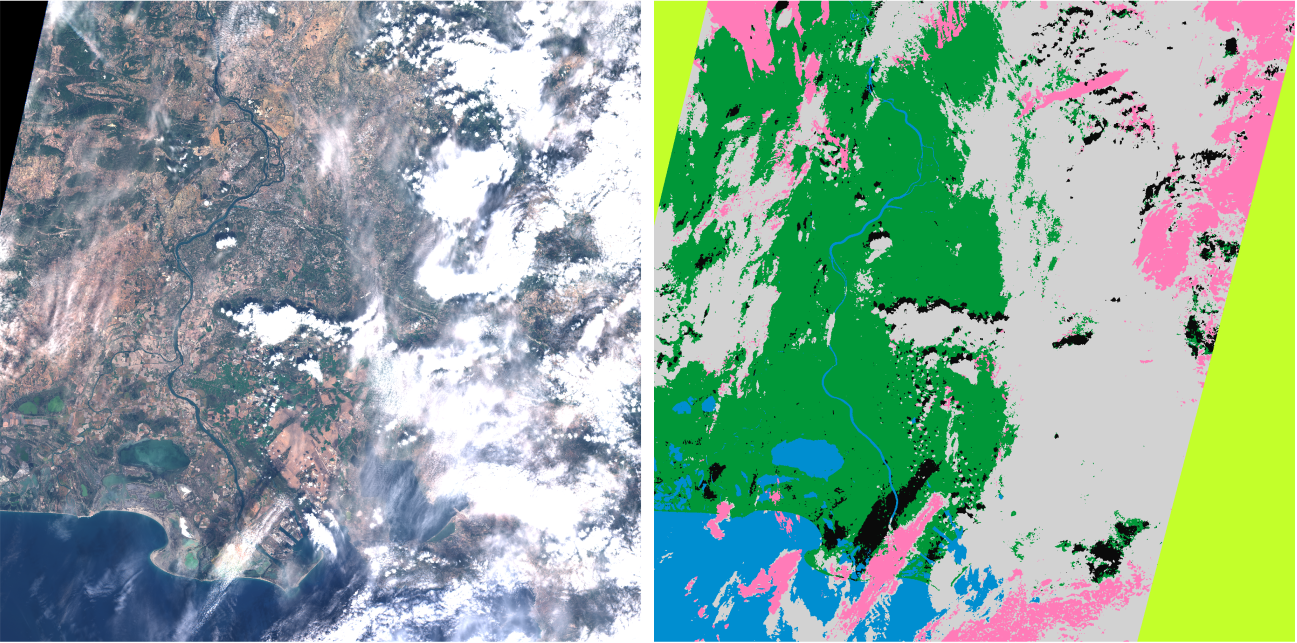
Figure 1: Classification of Arles, 20171002

Change to the ALCD directory. The program that you should use is all_run_alcd.py. You can display the help with

python all_run_alcd.py −h

The available options are:

• l: the location. The spelling should be consistent with the names in the L1C directory (e.g. Pretoria or Orleans)

• d: the (cloudy) date that you want to classify (e.g. 20180319)

• c: the clear date that will help the classification (e.g. 20180321)

• f: if this is the first iteration or not. If set to True, it will compute and create all the features, and create the empty class layers. Set it to True for the first iteration, and thereafter to False.

• s: the step you want to do, the choice is between 0 and 1. 0 will create all the needed files if this is the first iteration, otherwise it will save the previous iteration. 1 will run the ALCD algorithm, i.e train a model and classify the image. For each iteration, you should set it to 0, modify the masks, and then set it to 1.

• kfold: boolean. If set to True, ALCD will perform a k-fold cross-validation with the available samples.

• dates: boolean. If set to True, ALCD will display the available dates for the given location.

• global_parameters: path to json file which parametrize ALCD (for more information, please see the configuration documentation <configure_alcd.html#global-parameters>.)

• paths_parameters: path to json file which contain useful paths for ALCD (for more information, please see the configuration documentation <configure_alcd.html#paths-parameters>.)

• model_parameters: path to json file which contain classifier parameters (for more information, please see the configuration documentation <configure_alcd.html#model-parameters>.)

Paths preparation

Before running anything, you need to set the correct paths and parameters. In the paths_configuration.json:

• Add the tile code linked to the location you want to add

• Create the output directory for ALCD, and set its path in the “data_alcd” variable

• Set the correct paths for the L1C directory and the DTM_input. In the global_parameters.json, if you use a distant and a local machine, set the local_paths variables accordingly.

Step 1

A good practice is to visualise the two dates we want to use beforehand. This can be facilitated by the code quicklook_generator.py, which generates quicklooks for a given location. The user can therefore make sure that the cloud-free image is indeed cloud-free, and that the image to be classified is interesting. Therefore, initialize the environment by running :

python all_run_alcd.py -f True -s 0 -l city_name_dir -d cloudy_date -c clear_date -kfold False -global_parameters path_of_global_parameters.json -paths_parameters path_of_paths_configuration.json -model_parameters path_of_model_parameters.json

This will create the concatenated .tif with all the bands, and empty shapefiles for each class, among other things. It invites you to copy those created files to your local machine, to accelerate the process in QGIS (on our processing computer, visualisation is slow, so we use QGIS on a different computer). You can also modify the files directly, in this case, you can skip the manual copy of the files and go to Step 2. Otherwise, copy the files on your machine with QGIS, and go to Step 2.

Step 2

You can now open QGIS. Open the raster In_data/Image/city_name_bands_H.tif (H stands for Heavy, as it is in full resolution of 20m per pixel), and In_data/Image/city_name_bands.tif. The city_name_bands_H.tif bands refer to the band 2 (blue), 3 (green), 4 (red), 10 (the band at 1375nm), the NDVI and the NDWI. The bands for the city_name_bands.tif are quite numerous, but the content of each band is documented in the .txt file corresponding to each .tif. Now, adjust the style in QGIS such that you see the image in true colors. For that, you can load the file color_tables/heavy_tif_true_colors_style.qml on the Heavy .tif. You should get :

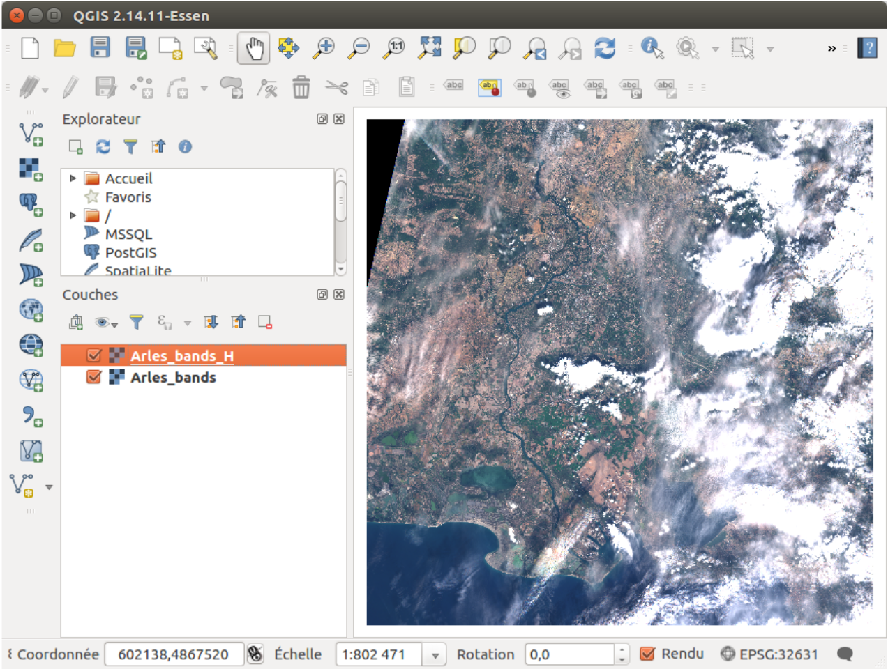
Figure 2: QGIS window with the scene displayed in true colors

Now, load all the empty shapefiles from the directory In_data/Masks. If you display a band being a time difference (for example the 20th band of city_name_bands. tif), you will observe that there was no data on the bottom-right corner for the clear date. The same is true with the top-left corner for the cloudy date. Thus, the no_data file already has some data (which is the case if one or both of the original images have no_data pixels). As you can see, on Figure 2 the top-left and bottom-right corners are covered by the no-data mask. If you are not satisfied with the mask, you can edit it manually. You should get something along the lines of the following :

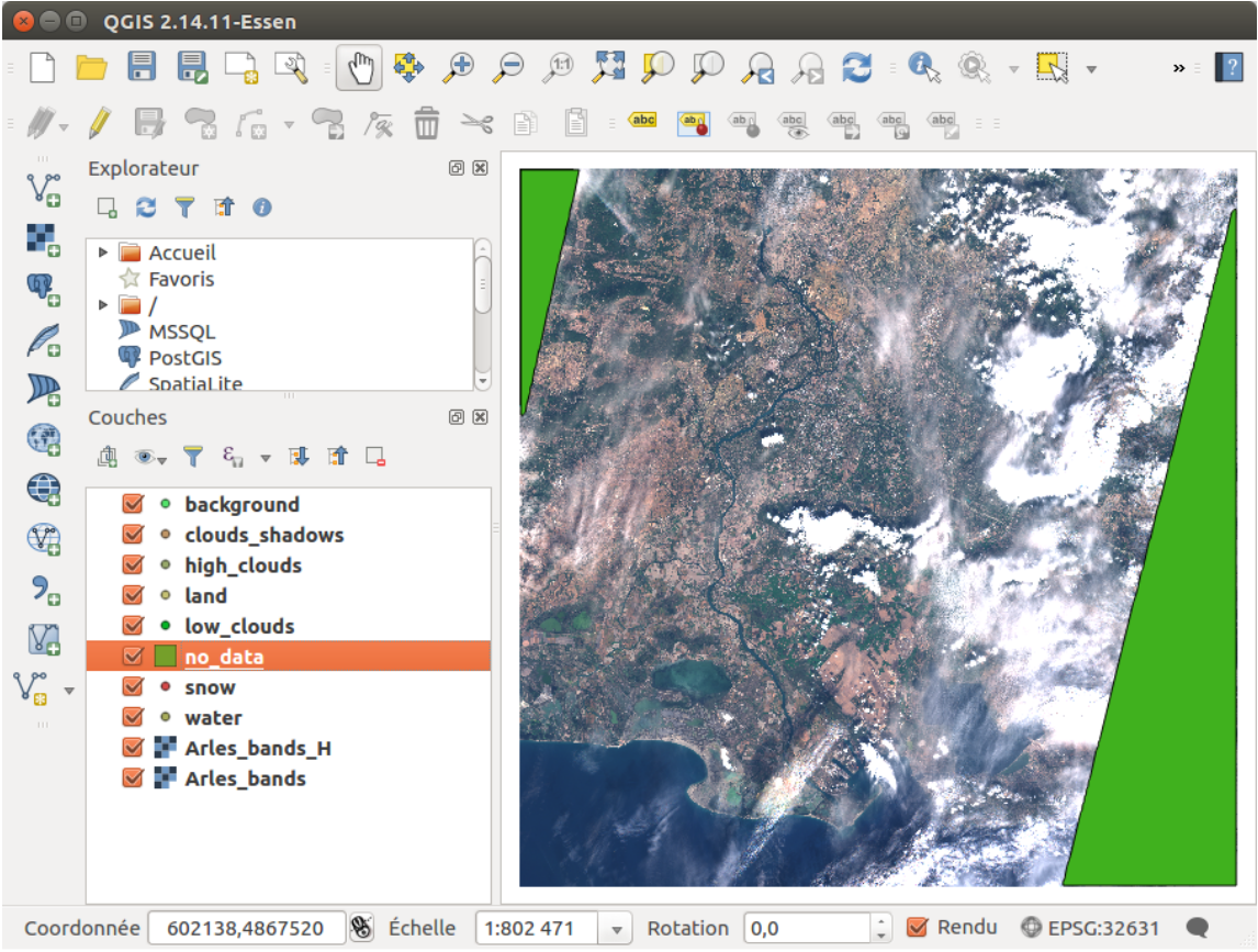
Figure 3: No-data areas are automatically computed

This no-data layer is used to discard the areas under it, be it for the classification, or if the user add samples in these areas by mistake.

Step 3

It is now time to edit the masks layers. For each class (land, low clouds, etc), edit the corresponding layer. Add the points that you want to take as samples, by clicking on the image and pressing Enter for each point. We have found more efficient to use points rather than polygons, we later dilate the points by 3 pixels assuming the neighbourhood is homogeneous in terms of class, so you should avoid to use a pixel just at the edge of a feature (cloud, land). The high clouds can be visible with the 1375nm band (i.e. the band number 4 of the heavy .tif). You can load the style heavy_tif_clouds_green_style.qml to see them quickly. The Figure 4 shows the image with the high clouds highlighted, and the steps to add points.

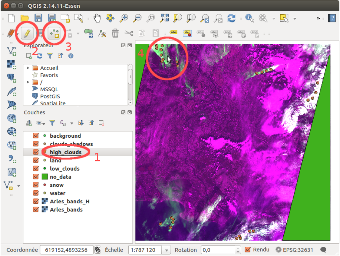
Figure 4: Steps to add data points with QGIS

Note

The 1375nm band is not to be trusted blindly. The principle of this band is that the water vapour in the atmosphere usually absorbs the photons in this wavelength. However, in dry conditions, or with high altitudes terrains (such as mountains), the photons can be reflected back. This can be misleading, so the user should take precautions. A typical way to detect such artefacts is to see if the potential cirrus shape is strongly correlated with that of the underlying terrain.

You can now go back to true colors, and continue by editing all the wanted classes. The background class can be used if you do not want to discriminate between land and water for example, but its use is not recommended. At the end, you obtain Figure 5

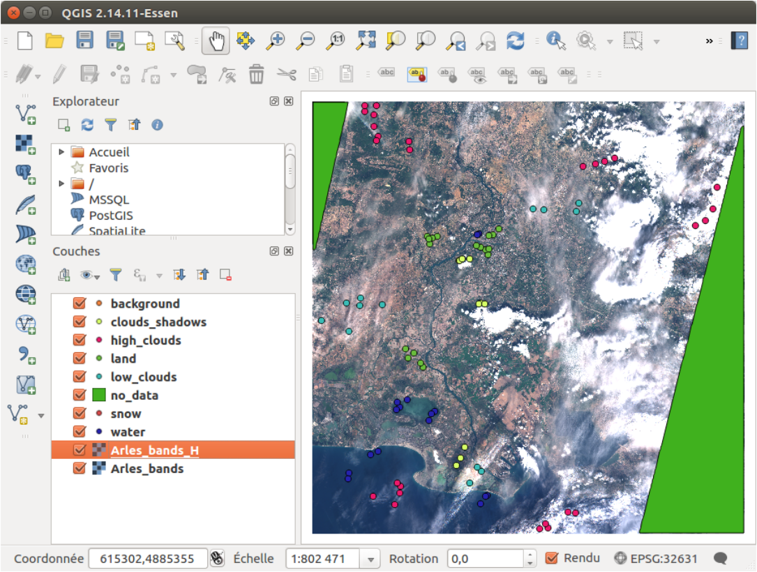
Figure 5: Samples placed manually after the first iteration

Step 4

Now, copy back the edited masks to the distant machine, or skip this if you work on one machine. It is time to train the model, and classify the image! Do it with :

python all_run_alcd.py -f True -s 1 -l city_name_dir -d cloudy_date -c clear_date -kfold False -global_parameters path_of_global_parameters.json -paths_parameters path_of_paths_configuration.json -model_parameters path_of_model_parameters.json

The results can be seen in the Out directory. The regularized classification map is labeled_ img_regular.tif. You can also see the contingency table in the Statistics directory. As you can see on the classification map, figure 2.8, some pixels are not well classified. Moreover, the confidence is low in numerous places, as seen on Figure 6. Therefore, we will take part of the advantage of this program: the active learning.

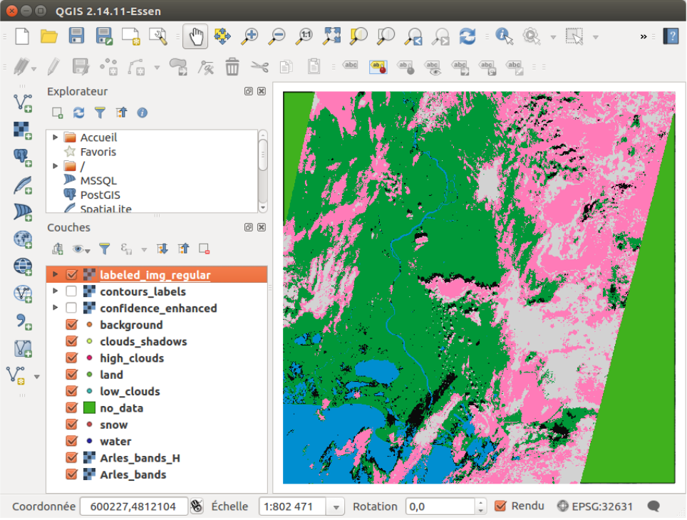
Figure 6: Result of the first classification

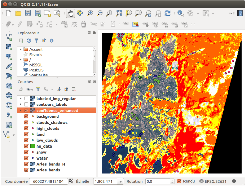
Figure 7: Confidence map of the first classification

Step 5

Do an new iteration, by running :

python all_run_alcd.py -f False -s 0 -l city_name_dir -d cloudy_date -c clear_date -kfold False -global_parameters path_of_global_parameters.json -paths_parameters path_of_paths_configuration.json -model_parameters path_of_model_parameters.json

It will save the previous iteration, and you can now edit the class layers, by adding new points (and also remove some if you made an error previously). You can copy on your local machine the outputs of the previous iteration (the bash command is given when you run the command above).

We suggest to open the files Out/contours_labels.tif and Out/labeled_img_regular. tif, and to apply to them the contours_labeled_contrasted_style.qml and the labeled_img_regular_style.qml styles respectively. It gives each class a recognisable color, which are given in table 1.

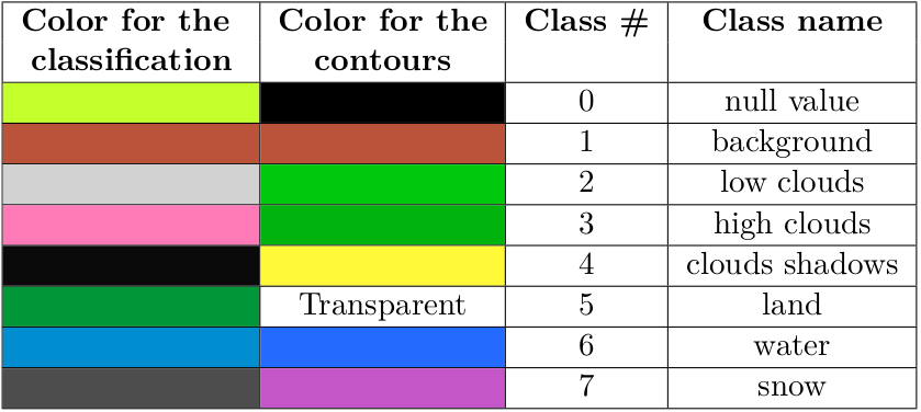
Table 1: Available classes and colors

For example, you can display the contours of the classes to see were the classifier was wrong. Here, we obtained a false detection of clouds shadows on the left of the image, which can be seen with the yellow contours:

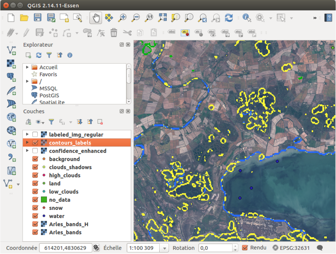
Figure 8: Contours of the shadows, in yellow

Therefore, we will add some points of land class in this region to increase the accuracy of our output, as shown in Figure 9.

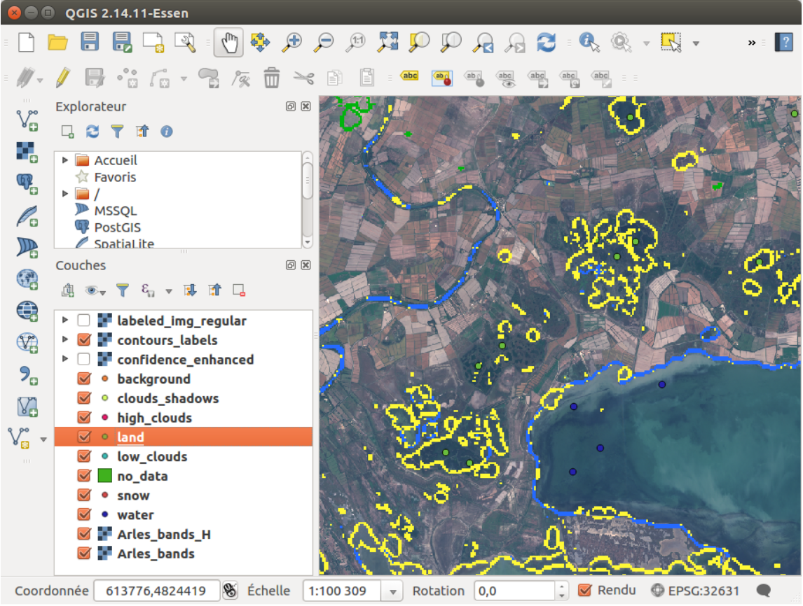
Figure 9: Some land samples are added where the wrong classification is visible

Do this for the areas where a misclassification is visible. Once the wanted points in each class have been added, you can copy back the layers to the distant machine with the appropriate command. Finally, you run once again the training and the classification with :

python all_run_alcd.py -f False -s 1 -l city_name_dir -d cloudy_date -c clear_date -kfold False -global_parameters path_of_global_parameters.json -paths_parameters path_of_paths_configuration.json -model_parameters path_of_model_parameters.json

Step 6

Repeat the Step 5 until you are satisfied with the classification the ALCD algorithm returns.

Quick tip: some data (30% by default) are used for the validation of the model, i.e. just to compute statistics. If you want to have more samples that you add manually to be taken into account for the training part, you can increase the training_proportion in the global_parameters.json.

Here is an example of the classification that you could obtain after each iteration. The 6th one is considered to be good (by myself), so you can stop there.

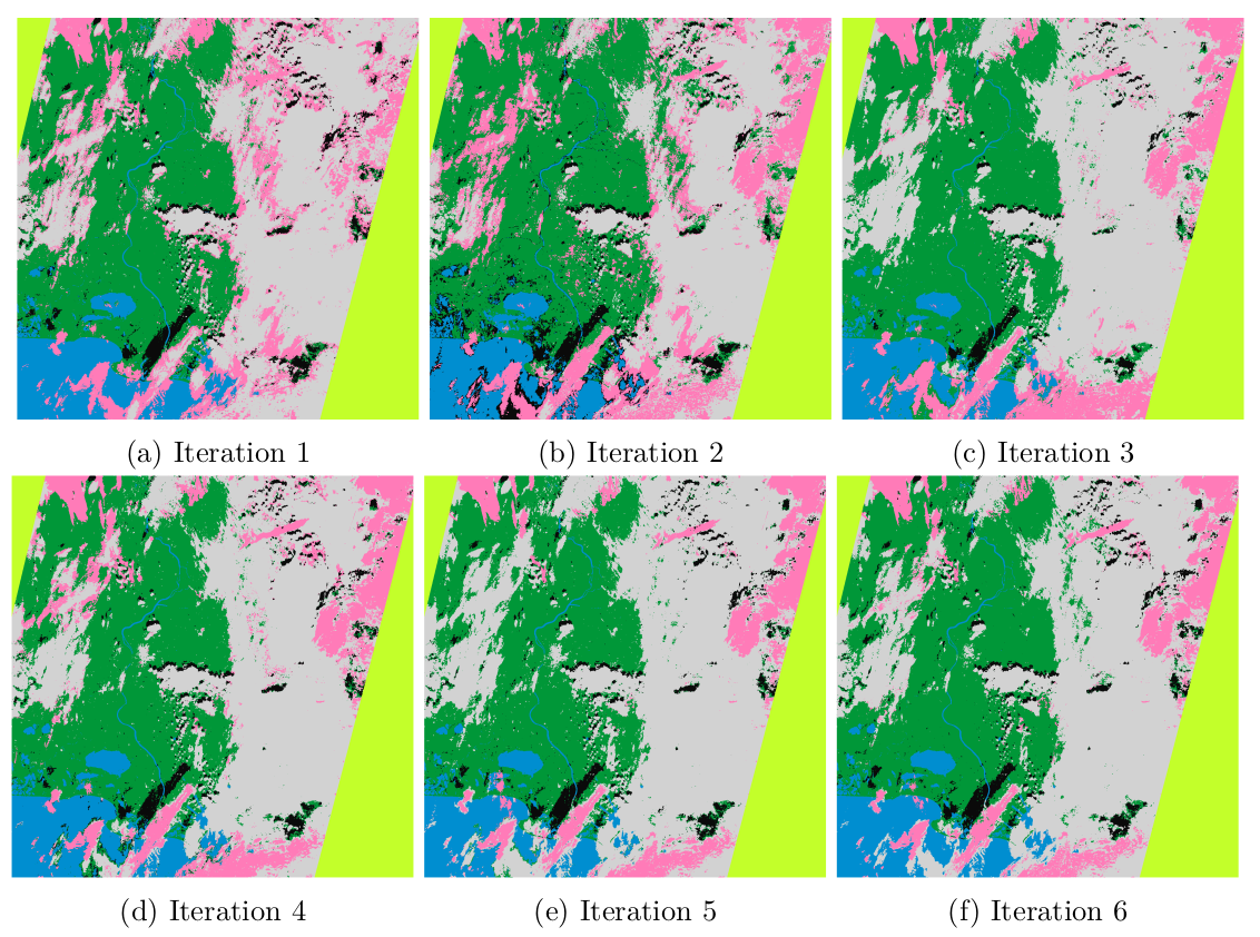
Figure 10: Evolution of the classification

As a reference, the QGIS windows at the last iteration with all the samples, with the labeled classification, and with the confidence map, are given in Figures 11, 12 and 13.

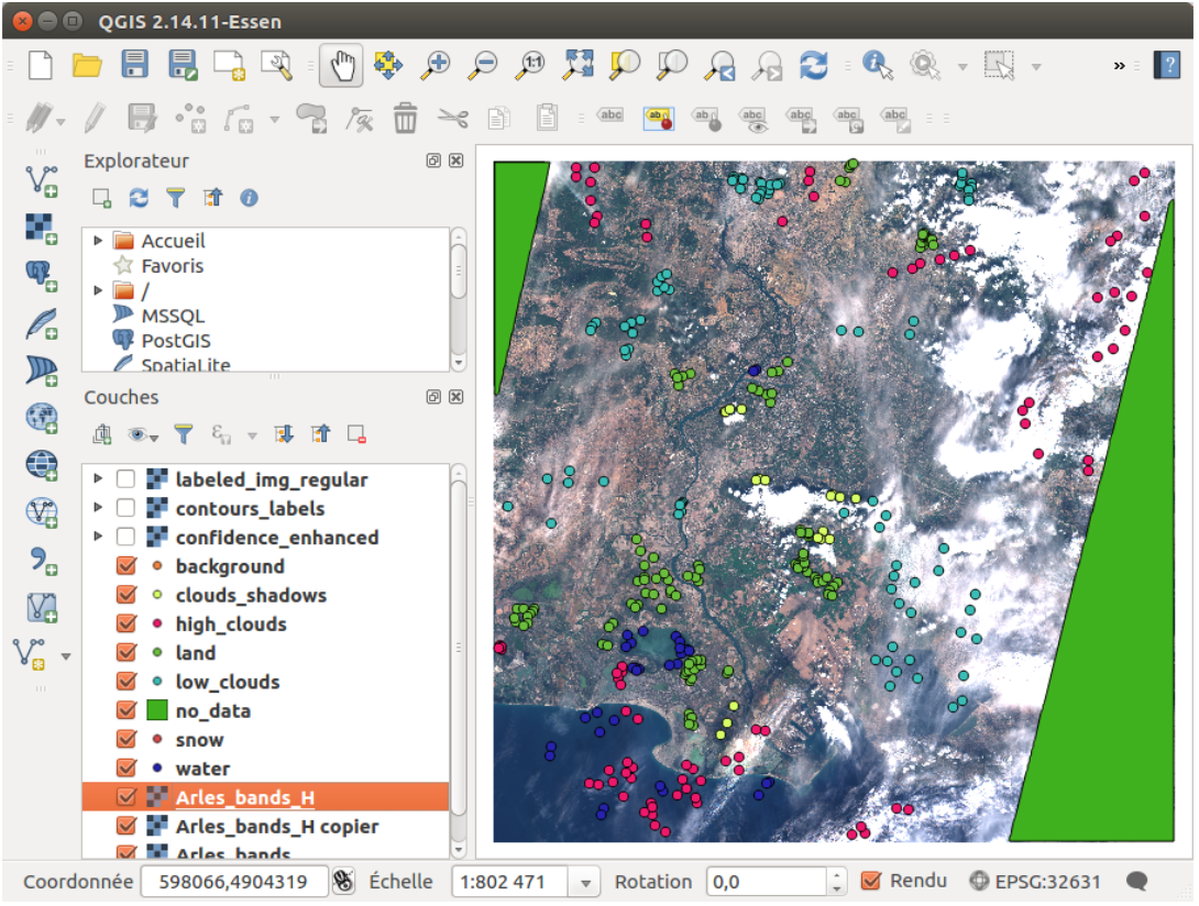
Figure 11: All samples present for the last iteration

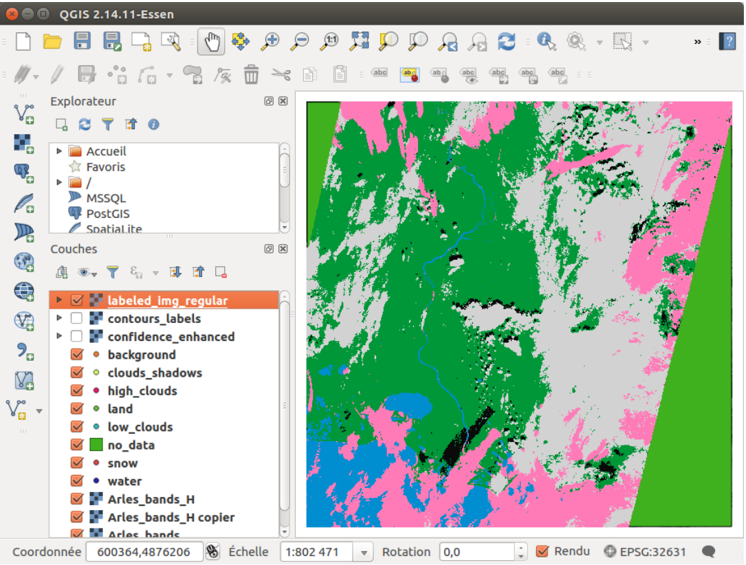
Figure 12: Labeled classification as seen in QGIS window for the last iteration

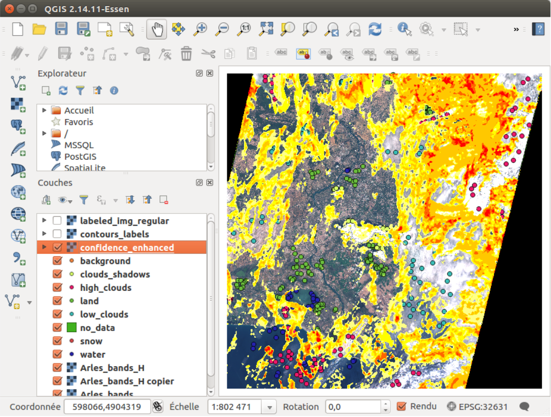
Figure 13: Confidence map as seen in QGIS for the last iteration