Cloud detection around montreux city
Introducing the inputs
ALCD requires several types of data for its execution
raster data on which the classification iterations will be performed.
json files to parameterise the chain.
The following sections will focus on the presentation of this data.
input rasters
ALCD currently only works with Sentinel-2 L1C data. However, it will be shown in the Custom stack section that it is possible to make ALCD use any type of data, as long as it is georeferenced.
Sentinel-2 L1C data can be download at: https://browser.dataspace.copernicus.eu
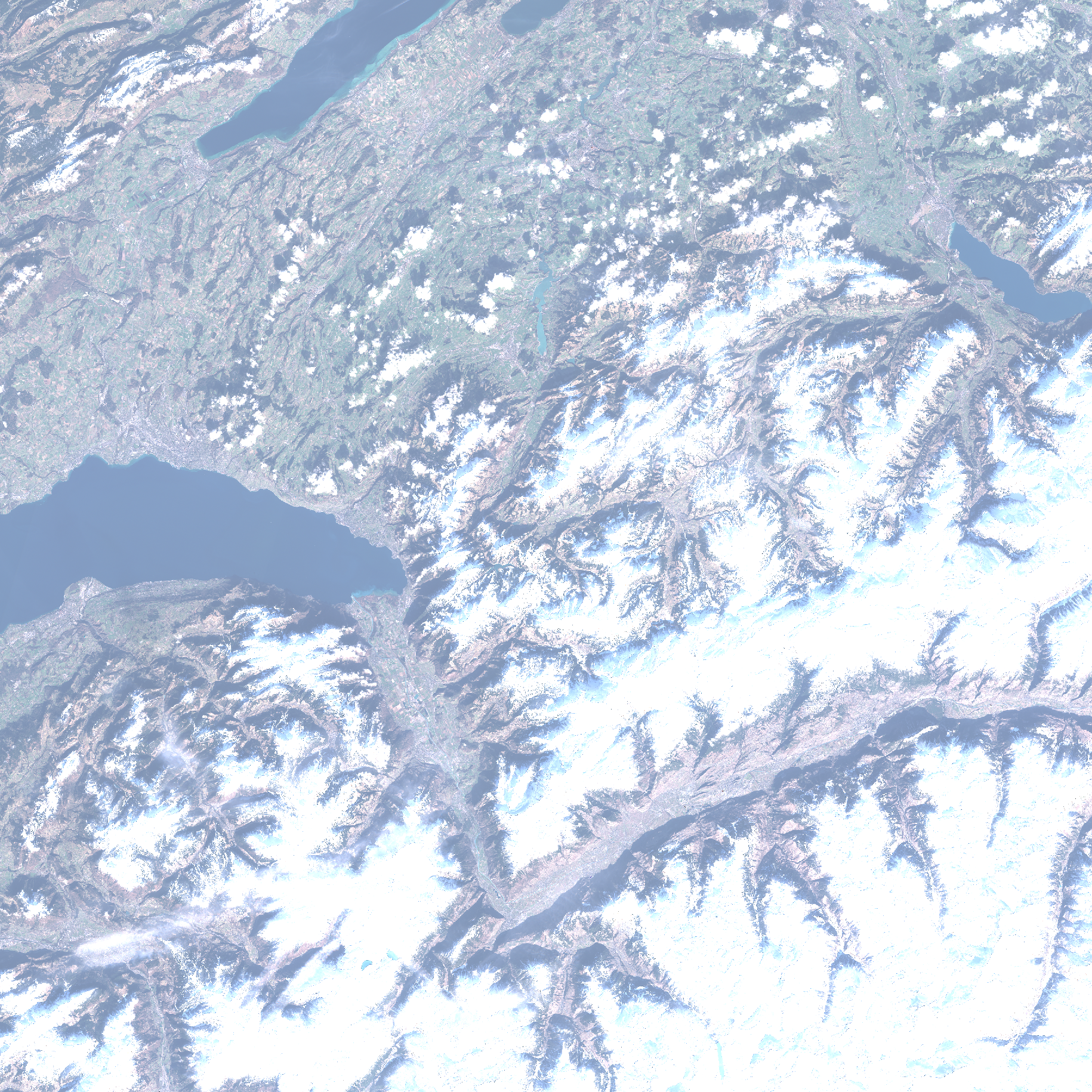
For the rest of this tutorial, we will use data acquired by Sentinel-2 on 13/02/2024 centred on the town of Montreux in Switzerland.
This data will be stored in the directory data_directory and must have a particular tree structure, organised by scene. For example, the Montreux scene must contain Sentinel-2 data for different dates.
from pathlib import Path
from utils import show_tree

data_directory = Path("./s2")
show_tree(data_directory)
Let’s take a look at the data.
from utils import show_raster

s2_20241302_r = data_directory/"Montreux"/"S2A_MSIL1C_20240213T103141_N0510_R108_T32TLS_20240213T141145.SAFE"/"GRANULE"/"L1C_T32TLS_A045150_20240213T103555"/"IMG_DATA"/"T32TLS_20240213T103141_B04.jp2"
s2_20241302_g = data_directory/"Montreux"/"S2A_MSIL1C_20240213T103141_N0510_R108_T32TLS_20240213T141145.SAFE"/"GRANULE"/"L1C_T32TLS_A045150_20240213T103555"/"IMG_DATA"/"T32TLS_20240213T103141_B03.jp2"
s2_20241302_b = data_directory/"Montreux"/"S2A_MSIL1C_20240213T103141_N0510_R108_T32TLS_20240213T141145.SAFE"/"GRANULE"/"L1C_T32TLS_A045150_20240213T103555"/"IMG_DATA"/"T32TLS_20240213T103141_B02.jp2"

show_raster(s2_20241302_r, s2_20241302_g, s2_20241302_b)
The RGB visualisation shows us the presence of clouds in the upper section of the image, but also snow in the mountains. Confusing clouds with snow is a common occurrence in machine learning.
Now that the data is stored in the expected tree structure, we can review the ALCD launch parameters
ALCD launching parameters
ALCD is launched using the python script all_run_alcd.py.
The available options are:
l: the location. The spelling should be consistent with the names in the L1C directory (e.g. Pretoria or Orleans)d: the (cloudy) date that you want to classify (e.g. 20180319)c: the clear date that will help the classification (e.g. 20180321)f: if this is the first iteration or not. If set to True, it will compute and create all the features, and create the empty class layers. Set it to True for the first iteration, and thereafter to False.s: the step you want to do, the choice is between 0 and 1. 0 will create all the needed files if this is the first iteration, otherwise it will save the previous iteration. 1 will run the ALCD algorithm, i.e train a model and classify the image. For each iteration, you should set it to 0, modify the masks, and then set it to 1.kfold: boolean. If set to True, ALCD will perform a k-fold cross-validation with the available samples.dates: boolean. If set to True, ALCD will display the available dates for the given location.global_parameters: path to json file which parametrize ALCDpaths_parameters: path to json file which contain useful paths for ALCDmodel_parameters: path to json file which contain classifier parameters
The last 3 parameters are json files containing parameters relating to the various stages of ALCD (image reading, learning, etc.). The next section describes the parameters required to launch the processing chain.
Contents of the configuration files
The first configuration file we are going to describe is the one to be filled in with the model_parameters parameter.
model_parameters
An example is available model_parameters.json
This file contains the options to be used by ALCD for each classifier that can be used in the otb TrainVectorClassifier application. For example, the contents of the file could be :
{
   	"svm_otb" : {
		"k":"linear",
		"m" : "csvc",
		"c" : "1",
		"opt" : "false",
		"prob" : "false",
        "rand" : "42"
	},
   	"rf_otb" : {
		"max":"25",
		"min" : "25",
		"ra":"0",
		"cat" : "10",
		"var" : "0",
		"nbtrees":"100",
		"acc" : "0.01",
        "rand" : "42"
	},
}
In this example, if the rf algorithm is selected then 100 trees will be used etc. For an exhaustive list of parameters, see the otb TrainVectorClassifier documentation.
paths_parameters
An example is available paths_configuration.json
This file contains the following information
{
   "data_paths": {
      "data_alcd": "montreux_outputs"
   },
   "global_chains_paths": {
      "L1C": "s2"
   },
   "tile_location": {
      "Montreux": "32TLS"
   }
}
data_alcd: must point to an output directory.L1C: must point to the Sentinel-2 data where the tree structure described in input rasters is respected.tile_locationallows you to select one of the scenes in the directory pointed to byL1C. In our caseMontreux. The per-scene field is used to create the output directory. The output directory is constructed as follows: ‘tile_location.key’_‘tile_location.key.value’_date where date is the date selected in the command line.
global_parameters
An example is available global_parameters.json.
This file contains the parameters for the various algorithms used. For example, this is the place where the classifier is chosen (rf, libsvm, etc.). We’ll focus here on the color_tables field.
{
   "color_tables": {
      "otb": "otb_table.txt"
   }
}
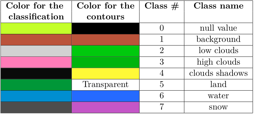
which must point to a text file containing the RGB information for each of the classes. It is this colour table that will be used to create the final classifications. Here is en example with 3 classes :
# Lines beginning with a # are ignored
# class R G B
0 195 255 42
# background
1 187 83 58
# low clouds
2 210 210 210
ALCD’s first launch on the scene
Launching command
Now that the configuration files have been filled in, we can launch the first stage of ALCD, which will create
- the ALCD output directories
- the stack of primitives
- the empty database required for training purposes.
To launch this preliminary stage, we need to use the following launch options
force True: to overwrite existing files
s 0: to launch the first stage.
f True: tells ALCD that this is not a new iteration. ‘f’ meaning ’first step ?
l Montreux: selects the scene to be processed (location)
d 20240213: the date to use in the available scene
c 20240213: the clear date to be used for the available scene. If no date available, can be equal to d.
kfold False: do not perform kfold learning.
%%bash
export PATH_ALCD="../../.."
python $PATH_ALCD/all_run_alcd.py -force True -s 0 -f True -l Montreux -d 20240213 -c 20240213 -dates False -kfold False -global_parameters global_parameters.json -paths_parameters paths_configuration.json -model_parameters model_parameters.json > tuto_log.txt 2>/dev/null
Results analysis
When the command has finished, the results should be present in the output directory with the following tree structure
from pathlib import Path
from utils import show_tree

data_directory = Path("./montreux_outputs")
show_tree(data_directory)
In_data/ImageContains the feature stacks that can be used during training. The .txt versions show which band corresponds to which feature in theIntermediatedirectory.In_data/MasksContains the empty databases representing the model’s learning points. By default ALCD offers: background, clouds_shadows, high_clouds, land, low_clouds, snow, water and no_data.IntermediateContains the feature used to build the stacks present in In_data/Image.
Launching the next stages
Before launching the following actions must be taken by the user:
modify the configuration file
global_parameters.json.update the databases previously created by ALCD.
Update global_parameters.json
the user_choices section needs updating, particularly the main_dir and raw_img fields, which represent respectively where the feature stack are stored and their names.
{
   "user_choices": {
      "main_dir": "montreux_outputs/Montreux_32TLS_20240213",
      "raw_img": "Montreux_bands.tif"
   }
}
Update learning databases
As seen above, ALCD has created empty learning databases, in In_data/Masks, for each of the desired classes. It is up to the user to fill in these databases using visualisation tools such as Qgis or others.
Once the global_parameters.json file and the databases have been updated, we can launch the rest of the processing.
Launching command
The command to run is almost identical to the previous one, except that the s option changes from 0 to 1.
%%bash
export PATH_ALCD="../../.."
python $PATH_ALCD/all_run_alcd.py -force True -s 1 -f True -l Montreux -d 20240213 -c 20240213 -dates False -kfold False -global_parameters global_parameters.json -paths_parameters paths_configuration.json -model_parameters model_parameters.json > tuto_log.txt 2>/dev/null
Results analysis
When the command has finished, the results should be present in the output directory with the following tree structure
from pathlib import Path
from utils import show_tree

data_directory = Path("./montreux_outputs")
show_tree(data_directory)
The final results are all stored in the /Out directory
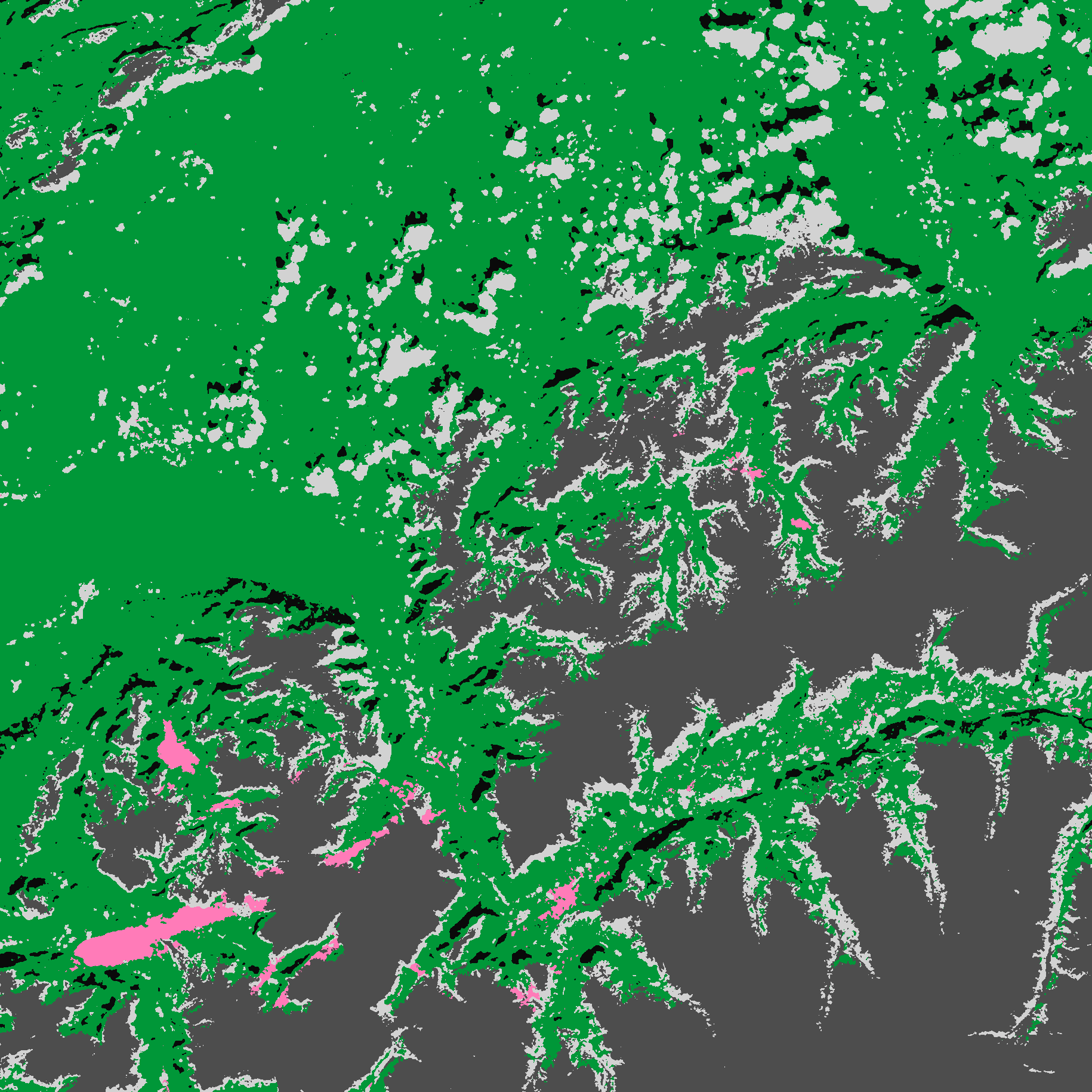
colorized_classif.png: the final classification with a different colour for each classconfidence.tifconfidence mapconfidence_enhanced.tif: confidence map averaged over a window of radius 11labeled_img.tif: final classificationlabeled_img_regular.tiffinal classification regularised in a window of radius 2.contours_labels.tif: contour mapcontours_superposition.png: quicklook of the contours map superimposed on the image to be classified.Quicklook.png: quicklook acquisition to be classified.
Here are the results after the first classification by ALCD.
from IPython.display import Image, display
display(Image(filename="montreux_outputs/Montreux_32TLS_20240213/Out/quicklook.png"))
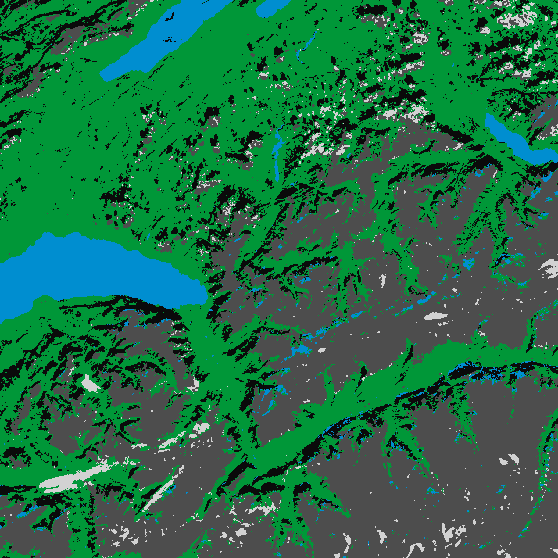
display(Image(filename="montreux_outputs/Montreux_32TLS_20240213/Out/colorized_classif.png"))
display(Image(filename="../images/table.png"))
Start next iteration
If the results are not satisfactory, it is possible to re-train by updating the training database. Before doing this, you need to save what was done previously with the command
%%bash
# considering PATH_ALCD is the path to the script 'all_run_alcd.py'
export PATH_ALCD="../../.."
python $PATH_ALCD/all_run_alcd.py -force False -s 0 -f False -l Montreux -d 20240213 -c 20240213 -dates False -kfold False -global_parameters global_parameters.json -paths_parameters paths_configuration.json -model_parameters model_parameters.json > tuto_log.txt 2>/dev/null
The use of -s 0 -f False triggers a copy of the previous run in the Previous_iterations directory, which was initially empty. This backup can be used to track the evolution of classifications over the course of iterations.
After this command has been run, it is possible to modify the initial training database. In our case, the results for water were disappointing. We will add water samples.
Then run ALCD again with the command
%%bash
# considering PATH_ALCD is the path to the script 'all_run_alcd.py'
export PATH_ALCD="../../.."
python $PATH_ALCD/all_run_alcd.py -force False -s 1 -f False -l Montreux -d 20240213 -c 20240213 -dates False -kfold False -global_parameters global_parameters.json -paths_parameters paths_configuration.json -model_parameters model_parameters.json > log_tuto.txt  2>/dev/null
The results generated during this iteration overwrite the previous ones. With the addition of samples, we can see an evolution in the classification
display(Image(filename="../images/quicklook_2.png"))
display(Image(filename="../images/colorized_classif_2.png"))
display(Image(filename="../images/table.png"))
Advance usages
Custom stack
As we saw in at the beginning of the tutorial, the user must specify which features should be used to learn a model. For example, it is possible to change ALCD’s initial function from cloud detection to water detection using Sentinel-1 images.
All the user has to do is place his own stack of features in the In_data/Image directory and enter its name in the global_parameters.json Json file in the user_choices.raw_img field.
Class definition
The classes to be used during ALCD execution are defined in the Json file global_parameters.json, in the masks section.
An example of classes is shown below.
"masks": {
      "background": {
         "class": "1",
         "shp": "background.shp"
      },
      "clouds_shadows": {
         "class": "4",
         "shp": "clouds_shadows.shp"
      },
      "high_clouds": {
         "class": "3",
         "shp": "high_clouds.shp"
      }
   }
There are 3 classes with their representation in the form of a character string, an integer and the file which will contain the database for this class.
If we want to add a forest class, then the file will contain
"masks": {
      "background": {
         "class": "1",
         "shp": "background.shp"
      },
      "clouds_shadows": {
         "class": "4",
         "shp": "clouds_shadows.shp"
      },
      "high_clouds": {
         "class": "3",
         "shp": "high_clouds.shp"
      },
      "forest": {
         "class": "4",
         "shp": "forest.shp"
      },
   }
Other classification algorithms
The user can choose the classification algorithm by modifying the “method” field in the global_parameters.json “classification” section.
Classification can be performed using either Orfeo ToolBox (OTB) or scikit-learn, the following algorithms are available :
-
Random Forest, “method”: “rf_otb”
SVM, “method”: “svm_otb”
Boosting, “method”: “boost_otb”
Decision Tree, “method”: “dt_otb”
Gradient Boosted Tree, “method”: “gbt_otb”
K-Nearest Neighbors, “method”: “knn_otb”
-
Random Forest, “method”: “rf_scikit”
SVM, “method”: “svm_scikit”
AdaBoost, “method”: “ada_scikit”
Extra trees, “method”: “xtree_scikit”
Gradient Boosting, “method”: “grad_scikit”
Histogram-based Gradient Boosting, “method”: “hist_grad_scikit”
The parameters for the choosen algorithm can be changed in the model_parameters.json file as explained in previous sections. As an example, when the AdaBoost classifier from scikit-learn is choosen, the user can enter the desired values for the parameters of the sklearn.ensemble.AdaBoostClassifier(estimator=None, n_estimators=50, learning_rate=1.0, algorithm=‘SAMME.R’, random_state=None) function :
"ada_scikit" : {
		"n_estimators" : 100,
		"learning_rate" : 1.0,
		"random_state" : 42
	},
User features
Users can integrate custom processes to modify the input data before classification by adding “user_function” and “user_module” fields in the “user_choices” section of the global_parameters.json file:
"user_choices": {
    "user_module": "tests/data/users_function.py", //Path to the Python file containing the user's process
    "user_function": "my_process", //Name of the function to apply
    //Other fields to specify
}
The custom function accepts a xarray.DataArray as input and return the modified xarray.DataArray.
This allows users to add or remove bands, compute indices, or perform any other transformations. For example, a function can remove bands and compute indices such as NDSI and add them to the input data. Below is a example from tests/users_function.py:
def my_process(in_tab : xr.DataArray) -> xr.DataArray :
    """
    Computes the NDSI of the input image
    """
    new_band =  (in_tab.loc['B03'] - in_tab.loc['B11']) / (in_tab.loc['B03'] + in_tab.loc['B11'])

    # band_list = list(in_tab.coords['band'].values)
    # band_list.remove("B01")
    band_list = ['B02', 'B03', 'B04', 'B08', 'NDVI', 'NDWI']

    out_tab = in_tab.sel(band=band_list)
    out_tab = xr.concat(
        [
            out_tab,
            new_band.expand_dims(band=["NDSI"]),
        ], dim='band',
    )
    return out_tab
If no modifications to the input data are needed, remove the “user_function” and “user_module” fields from global_parameters.json.
If updates have been added to the user function, re-run the first stage with the following command after making the changes :
python $PATH_ALCD/all_run_alcd.py -force True -s 0 -f True -l Montreux -d 20240213 -c 20240213 -dates False -kfold False -global_parameters global_parameters.json -paths_parameters paths_configuration.json -model_parameters model_parameters.json > tuto_log.txt
This ensures that the new function has been correctly applied to the input data.